Fluid Physics
8.292J/12.330J
Problem Set 4
Solutions
1. Consider the problem of a two-dimensional (infinitely long) airplane wing traveling in the negative x direction at a speed c through an Euler fluid. In the frame of reference of the airplane, the steady flow around the wind looks like

The
wing has width L and the flow over its upper surface can be characterized by a
speed ut, while under the lower surface it has a speed ub.
Since the upper surface is more curved than the lower surface, ut
> ub. The flow has a uniform density and you may neglect gravity in this problem.
a.) Derive an expression for the lift on the wing, per unit length in the y direction. (Hint: Consider the pressure acting on the lower and upper surfaces of the wing.)
Solution: The force per unit length in the y direction is just the pressure multiplied by L.
Thus the net upward force is just
|
|
|
From Bernoulli's equation for an Euler fluid,
|
|
|
where
is the ambient fluid pressure. Combining the
two expression above gives
|
|
|
b.) In the limit that the flow speeds ut and ub are not very different from c, show that the lift per unit length is proportional to the circulation around the wing, with circulation defined, as usual,
,
where
is a unit vector along the wing surface.
Solution: From the answer to a, we can write
|
|
|
where
is the average velocity, which, if ut
and ub are not very different from c, is itself approximately equal
to c.
c.) The oncoming flow is irrotational. What can you deduce about the lift of an airplane wing moving through an Euler fluid?
Solution: By Stokes theorem, the circulation is the integral of the vorticity over the area enclosed by the curve. If the oncoming flow is irrotational, it follows that it has no vorticity and, in an inviscid fluid, incompressible fluid, there is no way for it to acquire any. We have apparently proven that airplanes and birds cannot fly: No circulation, no lift. This is known as D'Alembert's Paradox, named after Jean Le Rond d'Alembert (1717-1783), who performed a series of experiments to measure the drag on a sphere in a flowing fluid, and on the basis of the potential flow analysis he expected that the force would approach zero as the viscosity of the fluid approached zero. His experiments disproved this idea. The trick here is to realize that real fluids always contain some viscosity, which, no matter how small, causes the fluid in immediate contact with a rigid surface (such as an airplane wing) to come to rest with respect to that surface. Since the fluid far from the surface is moving, this implies the existence of vorticity in the intervening layer. As the viscosity vanishes, so too does the thickness of this boundary layer, and the vorticity within the boundary layer becomes very large, so that the product of the vorticity and the boundary layer depth remains finite. Thus real wings do generate vorticity and circulation.
2.
Much
of the circulation of the ocean is driven by the frictional stress exerted on
its surface by the wind. The essential dynamics can be understood using the
vorticity equation for an incompressible fluid. Including the effect of a turbulent
momentum flux, ,
in the vertical direction, this equation is
|
|
|
(1) |
where
is the vorticity. In the ocean, the vorticity
is strongly dominated by its vertical component, and the vertical component of
(1) can be written, to a very good approximation, as
|
|
|
(2) |
where
is the vertical component of velocity and
is a unit vector in the vertical direction.
If we approximate the flow of the ocean as steady, then
|
|
|
(3) |
and using this, (2) becomes
|
|
|
(4) |
Now we are interested in flow relative to the rotating earth. From the point of view of an observer in an inertial reference frame, the vertical component of the vorticity can be written
|
|
|
(5) |
where
is the earth-relative velocity (i.e. the
velocity we are interested in),
is the angular velocity of the earth, and
is latitude. The second term in (5) is just
twice the projection of the earth's angular velocity vector onto the local
vertical plane, and over most of the ocean, it is substantially larger in
magnitude than the first term on the right of (5).
Next
we substitute (5) into (4) and linearize the result about a state of rest ( =0), with the result that
|
|
|
(6) |
where
a is the radius of the earth, and is the south-to-north earth-relative velocity
component. Finally, for simplicity, we consider a range of latitude that is
small enough that we can neglect the variability of the coefficients of (6)
with latitude. Using the definitions
|
|
|
|
|
|
|
|
where
is some mean latitude, we can further
approximate (6) as
|
|
|
Equation (7) says that sources of vorticity owing to stretching and to wind stress at the surface must be balanced by north-south flow, bringing in water with higher or lower rotation rates coming from higher or lower latitude. (Water at rest at the equator has no vertical component of rotation,
You are going to make some deductions using (7) and the incompressible mass conservation equation.
Consider
an idealized rectangular ocean basin of dimensions and depth H, phrased in Cartesian coordinates
x, y and z. The basin is assumed to be in the Northern Hemisphere, so that both
and
are positive. Take the southern boundary of
the basin to lie along
,
the northern boundary to lie along
,
the western boundary to lie along
,
and the eastern boundary to lie along
.
a.)
Assuming that the vertical velocity, ,
vanishes at both the top and bottom of the ocean, and that the wind stress also
vanishes at the bottom (but not the top!), integrate (7) over the whole depth
of the ocean to find an expression for the depth-averaged south-to-north
velocity,
.
Solution: The first term on the right of (7) integrates to zero, leaving
|
|
where is the surface stress.
b.)
Integrate the mass continuity equation for an incompressible fluid through the
depth of the ocean to find a differential relation between and the depth-averaged west-to-east velocity
component,
.
Solution: The mass continuity equation for an incompressible fluid is just
|
|
|
Integrating this with depth gives
|
|
where
is the depth-averaged west-to-east velocity
component.
c.)
The wind flow over the
|
|
where is the wind stress at the ocean surface and
is the amplitude of the wind stress curl.
Using
the result of (a) above, find an expression for .
Now using the result of (b) above, find an expression for
.
Note that the boundary condition on
is that it must vanish at both the eastern and
western boundaries. You will not be able to satisfy both of these conditions.
So find two solutions: one that satisfies
=0 on the eastern boundary, and one that
satisfies
=0 on the western boundary.
Solution: Using (10) in (8) gives
|
|
(11) |
while using this in (9) gives
|
|
(12) |
Integrating
this, subject to on the western boundary gives
|
|
while
if on the eastern boundary, we get
|
|
d.)
The reason that both boundary conditions on cannot be satisfied is that there exists at
either the western or the eastern boundary a thin boundary layer in which all
of the "return flow" is concentrated and in which some of the approximations
we used break down. The most important approximation is the neglect of the
friction of the ocean flowing along the side boundaries. One effect of this
friction is to change the vorticity of the fluid. Note that the wind stress in
our problem provides a negative definite basin-averaged vorticity tendency. In
the steady state, this will have to be balanced by a source. Considering
qualitatively how the side boundary friction might affect vorticity, at which
boundary (east or west) do you think the return flow is concentrated? Explain your reasoning, and sketch what the
flow might look like (including the boundary layer).
Solution: If we add a boundary layer on the eastern boundary to the flow given by (13), the result looks something like
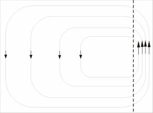
This solution cannot work, because friction along the eastern boundary would impart even more clockwise rotation to the fluid, in addition to that imparted by the clockwise wind in the interior of the ocean. Instead, the correct solution is (14), with a western boundary layer:
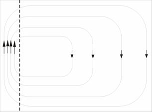
This
way, the western boundary imparts counterclockwise rotation to the fluid,
balancing that imparted by the wind. This is a simple model of the
Extra Credit: The effect of side boundary friction can be modeled by adding a term
|
|
|
|
to
the right-hand side of (2), where is a coefficient which you may assume is
constant. This term is negligible in the interior, where the solution we
obtained before is valid. But it dominates the right side of (2) in the thin
boundary layer. By obtaining a solution for the thin boundary layer and
matching this to the interior solution at the outer edge of the boundary layer,
find a solution that satisfies both boundary conditions on
and also satisfies
on the continental side of the boundary layer.
Solution: When the viscous stress term given above is added to the right-hand side of (2), the derivation leading to (7) instead gives
|
|
In the thin western boundary current, the last term above dominates over the wind stress, so that, when averaged over depth, (15) becomes, approximately,
|
|
If we define a viscous length scale
|
|
|
then the general solution of (16) is
|
|
(17) |
where A, B and C are integration constants.
These are determined by applying the following boundary conditions. First, at the western boundary (x=o) itself,
the velocity of a viscous fluid must vanish. Second, at the outer edge of the
boundary layer, ,
the velocity must match the interior velocity,
.
Finally, the flow integrated over the with of the boundary layer must be equal
in magnitude an opposite in sign to the velocity integrated over the interior
of the ocean basin, so that there is no net northward or southward flow of
mass:
|
|
(18) |
Applying these three conditions yields the integration constants. The solution looks qualitatively like the second figure above.