It is evident from the potential intensity climatology that there is no shortage of potential energy for tropical cyclones over much of the Tropics during much of the year. But tropical cyclones are rare...there are only about 80 of them every year, worldwide. The reason for this is that tropical cyclones don't start spontaneously, ``like a child from the womb, like a ghost from the tomb", as Shelley described the formation of ordinary clouds. It turns out that the normal tropical atmosphere is metastable to tropical cyclones...small perturbations die away, even when the environment is very conducive to genesis.
To demonstrate this important point, we can run a numerical simulation of a tropical cyclone and see what happens if we start with too weak a perturbation. Let's look at the numerical model by Rotunno and Emanuel (1987) [8]. This model solves the full equations for the conservation of momentum, heat and water in two phases, with liquid water divided into two categories: cloud droplets that move with the air, and raindrops that fall and can evaporate. The only approximations that are made in the equations themselves are assumptions predicated on the flow being substantially subsonic. The equations are integrated on an axisymmetric grid which runs every 7.5 km out to 1500 km in the radial direction, and every 1.25 km up to 25 km in the vertical. Motions on scales smaller than the grid size are represented in terms of resolved variables using a fairly sophisticated representation of turbulence, that depends on the rate of strain of the resolved flow and the stability to local convective overturning. Condensed cloud water is turned into rain at a specified rate, and the rain falls and can evaporate into subsaturated air. (There are no ice physics in the model.) Surface fluxes of heat, water and momentum are represented in terms of bulk aerodynamic formulae of the form (27), with the exchange coefficients for the three quantities assumed equal, although they are linear functions of surface wind speed to account for the dependence of the surface roughness on waves. The outer and upper boundaries are rigid walls, but since the equations admit internal buoyancy and rotation waves as solutions, something has to be done to prevent large reflections of such waves back into the domain. In this model, the outer and upper walls are lined with ``sponge layers", which are about 5 grid points thick. In these layers, linear damping terms are added to all the time-dependent equations, which have the effect of relaxing the quantities back toward their initial values. The coefficients of damping vary from zero just inside the sponge layers to their maximum values just inside the walls. These sponge layers absorb much, but not all of the wave energy incident on them.
Initializing tropical cyclone models is especially problematic. Ideally, one would like to begin with a background state in radiative-convective equilibrium. Radiation codes are very computationally expensive, so one short cut might be to simply specify a background radiative cooling profile and some surface heat fluxes, and let the model convect until it reaches a statistically steady state. The problem with this has to do with the imposed axisymmetry. Moist convection is a complex and highly three-dimensional form of turbulence. Normally, three-dimensional turbulence cascades energy from the scales at which it is generated down to very small scales, where it is finally dissipated by molecular diffusion. But, as shown by a famous theorem due to Fjortoft, when turbulence is forced into a two-dimensional straightjacket, it actually cascades energy upscale to the largest scales that will fit into the domain! This happens in axisymmetric tropical cyclone models, so that ordinary cumulus convection, forced by the symmetry of the model to assume the form of rings, rather than towers, of cloud, will artificially result in a vortex even if there are no other supporting physical processes.
For this reason, it is not feasible to begin from a state of radiative-convective equilibrium. In the model of Rotunno and Emanuel (1987) [8], the initial background state is one that is very nearly neutral to cumulus convection, with no radiative cooling at all. This neutral state is achieved by first performing a preliminary experiment starting from an unstable condition but without the earth's rotation included, so that no vortex can form. The model is allowed to convect until the convection has exhausted the supply of potential energy and thus dissipates. This neutralized thermodynamic state is then used as the background state for all subsequent integrations of the model. To represent the effects of the background convection and radiation that would occur in reality, all perturbations of temperature to this background state are relaxed back to zero over a time scale of about one-half day, but with the provision that the local cooling rate never exceed 2 K/day.
If the model is initialized with just this resting, background state, nothing happens. As there is no wind, there are no surface fluxes, and since there is no perturbation temperature, there is no atmospheric cooling. The atmosphere just sits there.
To get something going, a weak vortex is superposed on the background state. The vortex has the structure of a tropical cyclone, with a warm core and a surface cyclone diminishing in intensity with height. This initial vortex is exactly in gradient wind and hydrostatic balance, as given by (1) and (2).
Once the vortex is in place, surface friction begins to retard the wind near the surface, and at the same time, surface enthalpy fluxes begin to warm and moisten the boundary layer. When the surface wind speed diminishes, the radial pressure gradient, which is not directly affected, is no longer completely balanced by the outward-directed centrifugal and Coriolis forces, and air begins to accelerate inward, down the pressure gradient. By mass continuity, the inward flowing air must turn upward near the vortex center, giving rise to ascending motion there. (This process, by which friction acting on a cyclonic flow forces ascent, is called Ekman pumping). The ascending air cools adiabatically, destabilizing the column and promoting convection preferentially near the vortex center.
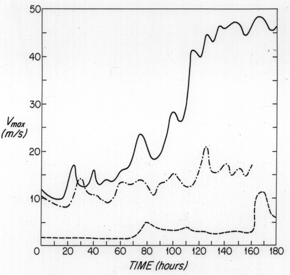
The evolution of the domain-maximum wind speed with time is shown in Figure 6.1
for three different numerical experiments. The first, labeled the control,
begins with a fairly small scale vortex with a maximum wind speed of  . Initially, it slowly decays, but after a few days, it begins to
amplify, and then rather quickly develops into a full-fledged model tropical
cyclone. It achieves a quasi-steady state that lasts for as long as one cares
to run the model. In class, we will look at various quantities, such as all
three velocity components, temperature and entropy, characterizing the mature
state of the model tropical cyclone.
. Initially, it slowly decays, but after a few days, it begins to
amplify, and then rather quickly develops into a full-fledged model tropical
cyclone. It achieves a quasi-steady state that lasts for as long as one cares
to run the model. In class, we will look at various quantities, such as all
three velocity components, temperature and entropy, characterizing the mature
state of the model tropical cyclone.
If one begins with a weak vortex, nothing much happens, even if the model is integrated for a very long time. This is shown by the second curve in Figure 6.1. Also, if the starting vortex is too large in horizontal scale, it does not develop (third curve in Figure 6.1). These experiments confirm what weather forecasters have known for a long time: tropical cyclones do not develop spontaneously in the tropical atmosphere, but require some kind of triggering disturbance to get them going. It is a good thing that this is the case, otherwise we might be plagued by frequent tropical cyclones.
So the tropical atmosphere is metastable to tropical cyclones. But why is this the case? This is one of the central problems in understanding the physics of tropical cyclones. Before tackling this problem, let's look at an observed case of tropical cyclone genesis.
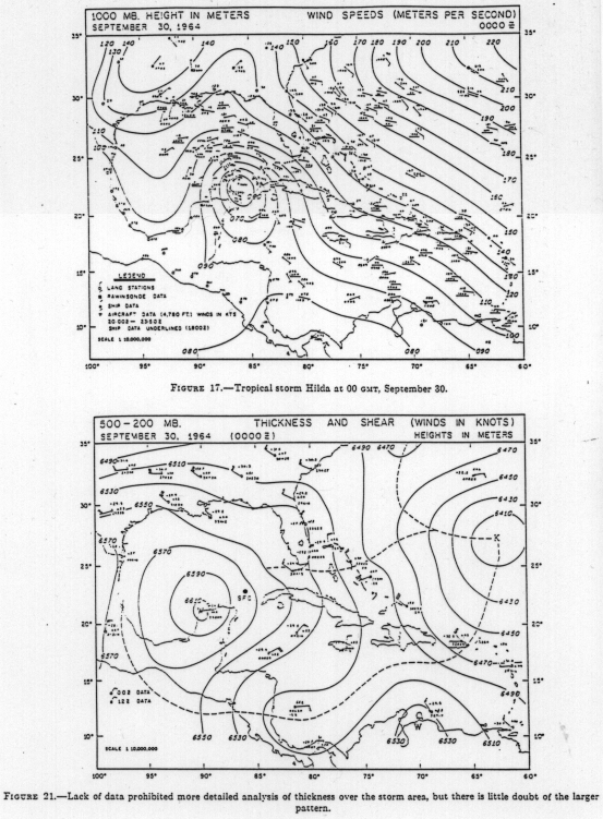
We choose as a case study the development of Hurricane Hilda in 1964. (One reason for choosing such and old case is that, hard as it may be to believe, we had somewhat more useable data in the 1950s and 1960s than we have today. There were quite a few rawindsonde stations scattered around the Caribbean and western North Atlantic region. A rawindsonde is a weather balloon that measures temperature, pressure, humidity and wind speed and direction. Today, the number of launch sites is diminishing, and there are only one or two launches per day; in the 1950s and 1960s some stations launched 3 times daily. To some extent, the loss of rawindsonde data has been compensated by the advent of measurements from satellites, but it is difficult to get detailed quantitative information about the atmosphere this way.)
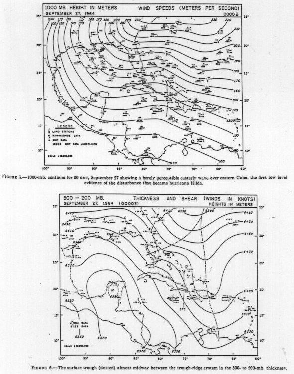
First examine Figure 6.2a. The top part of this figure (and subsequent ones in this sequence) shows contours of surface pressure over the Caribbean region up through Florida and the Gulf of Mexico. Generally, there is higher pressure to the north and lower pressure to the south. This is normal in the tropics, and is associated with geostrophic winds that blow from east to west. These are called the ``trade winds" as they enabled Europeans to sail easily to the New World and beyond. Also notice a wave in the isobars located south of eastern Cuba and Jamaica. This denotes a local ``valley", or trough, in the pressure distribution. This particular feature is called an easterly wave, a phenomenon that originates over eastern and central sub-Saharan Africa during summer, and which subsequently propagates westward over the North Atlantic. Easterly waves are very common in summer and are associated with passing showers. Now and then one will trigger a tropical cyclone, as this one did. The bottom of Figure 6.2a shows, at each rawindsonde station, the vector difference between the winds at 200 mb and the winds at 500 mb. The contours show the difference between the altitudes of the 200 mb and 500 mb pressure surfaces. This altitude difference is called the layer thickness and, according to the hydrostatic equation, (1), it is directly proportional to the average temperature in this layer. The 200 mb pressure surface is close to the tropical tropopause, so this layer is in the upper troposphere. Also, according to the thermal wind equation, the vector shear of the geostrophic wind in a given layer should be proportional to the magnitude of the horizontal thickness gradient in the layer, and its direction should be orthogonal to the direction of the thickness gradient. This relationship is well satisfied in the lower parts of figures 6.2a-d.
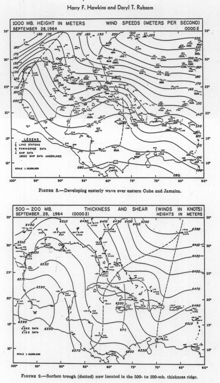
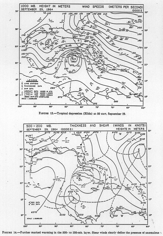
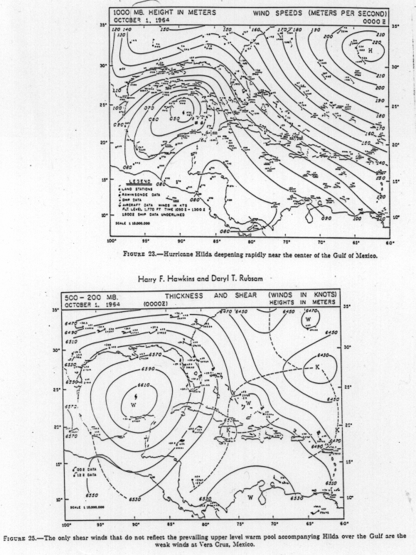
Notice a small amplitude trough in the 500-200 mb thickness and wind shear fields near Florida, in the bottom panel of Figure 6.2a. This represents a weak Rossby wave in the generally northwest-to-southeast flow of air at these high altitudes. We believe that the interaction between this wave and the lower tropospheric easterly wave in the upper panel of Figure 6.2a triggered to genesis of Hurricane Hilda. The subsequent evolution of the system, at 24 hour intervals, is shown in Figure 6.2b, Figure 6.2c, Figure 6.2d and Figure 6.2e. Note , in Figure 6.2b, that the upper trough is on collision course with the easterly wave and that the latter has amplified noticeably over the previous 24 hours. By the third day, Figure 6.2c, a tropical depression has formed, denoted by closed isobars at the surface, and at upper levels the first signs of the developing warm core are evident. It is about this time that the Carnot cycle is switched on and the true tropical cyclone dynamics take over. Notice in the subsequent development that the weak upper trough, having played out its role as a catalyst, is eaten alive by its easterly wave spouse, sharing the fate of the male black widow spider. The upper warm core, more or less collocated with the surface cyclone, rapidly becomes the dominant feature of the upper troposphere.
While the sequence of events shown in Figure 6.2 is by no means unusual, one should not conclude that this is the only way of triggering tropical cyclones. Many other modes of formation have been observed, about which more in due course.
One of the first questions one might ask about tropical cyclone genesis is, why do tropical cyclones need to be triggered? There should be a clue to the answer to this question in the numerical simulations described earlier in this lecture. After all, the numerical model also exhibits metastability to a resting atmosphere. The model has the enormous advantage of the easy availability of precise ``data". But, unless one is armed with a hypothesis to test, the behavior of a complex model can be as inscrutable as nature herself. Rather than to try to tackle the question of metastability with a complex model, we choose instead to build a ``stripped down" model that aims to be as simple as possible without being too simple. Using hierarchies of models of increasing complexity has many advantages when trying to understand physical systems.