A tropical cyclone is a rotating storm with typical horizontal scales of 100-1000 km and which extends through the depth of the troposphere, about 15 km. As its name implies, the sense of rotation is cyclonic...counterclockwise in the Northern Hemisphere and clockwise in the Southern Hemisphere. (As we shall see, the sense of rotation is reversed very near the top of the storm.) Some 85 tropical cyclones form worldwide every year. They are classified according to their maximum sustained wind speeds as follows (``maximum sustained wind speed" generally refers to the maximum 1 minute average wind speed recorded by an anemometer located 10 meters above the surface, though some countries use a 10-minute average):
 or less. but less than
  or greater.
This classification scheme is not universal but is used for North Atlantic and eastern North Pacific storms. A similar scheme is used in the western North Pacific region, except that ``typhoon" is used in place of ``hurricane". The word hurricane is derived from the Carib huricán, a God of evil, while ``typhoon" is thought to originate in the Arabic tufan, a violent storm of wind and rain, or the Chinese tai fung, ``big wind". (Note also that Typhon is Greek for whirlwind.)
Tropical cyclones originate over warm tropical ocean water, as can be seen in Figure 1.1, which shows the origin points of tropical cyclones over a 20 year period. There are three main belts of genesis activity: one covering the tropical North Atlantic, the Caribbean and Gulf of Mexico and extending westward across the eastern tropical North Pacific; another extending from about the dateline in the western North Pacific across the northern Indian Ocean, Bay of Bengal and the eastern Arabian Sea, and a third belt in the Southern Hemisphere from the tropical South Pacific, across northern Australia and the southern Indian Ocean as far west as the Malagasy Republic. No tropical cyclones form within about 5 degrees latitude of the equator, because their dynamics demand a non-trivial projection of the earth's rotation vector onto the local vertical. Also, curiously, there have never been reports of tropical cyclones anywhere in the South Atlantic.
Once formed, tropical cyclones tend to move westward and poleward. If they do not dissipate over land or cold water, they usually recurve poleward and eastward, often moving into middle and high latitudes before finally dissipating or transforming to extratropical cyclones which, unlike their tropical cousins, derive their energy from the potential energy stored in the pole-to-equator temperature gradient. Figure 1.2 shows the tracks of Atlantic tropical cyclones during the 1996 season. Tropical cyclones dissipate very quickly over land, with wind speeds falling below hurricane force typically in less than 12 hours. On the other hand, rainfall from tropical cyclone's can persist and even sometimes intensify many days after landfall, causing serious flooding. In rare cases, tropical cyclones rejuvenate over land by tapping into the baroclinic energy source resident in strong horizontal temperature gradients. When this happens, damage can occur well inland. An infamous case was Hurricane Hazel of 1954, which caused extensive damage in Toronto more than a day after landfall.
Figure 1.3 shows that tropical cyclones are creatures of the summer and early fall in both hemispheres. In the northwest Pacific basin, tropical cyclones can occur in any month of the year, though more occur in the summer. There is considerable interannual and interdecadel variability of tropical cyclone activity, and this is strongly related to other aspects of long term variability in the climate system. For example, long term variations in the tracks and numbers of Atlantic tropical cyclones are evidently related to drought cycles in the Sahel, as reported by Landsea and Gray (1992) [7] and shown in Figure 1.4 and Figure 1.5. (Figure 1.5 shows Atlantic tropical cyclone tracks classified according to how wet conditions are in the Sahel.) There is some indication that this variability is related to the North Atlantic Oscillation, which affects the sea surface temperature distribution. () have shown that North Atlantic tropical cyclones are strongly related to sea surface temperature distributions in a sector of the tropical Atlantic. In the Pacific region, the distribution of tropical cyclones is noticeably affected by the presence or absence of El Niño, with storms generally occurring further east in an El Niño year. Places such as Tahiti, which are almost never affected by tropical cyclones, may experience storms in an El Niño year. There is also some indication that storm activity is affected by the Madden-Julian oscillation, a wave-like oscillation that travels eastward around the equator with a period of around 40 days.
Although the basic structure of tropical cyclones is invariant, there is considerable variability in the both the details of the structure and the overall horizontal scale of the storms. In particular, the characteristic horizontal scale of tropical cyclones varies over a wide range, from ``midget typhoons", with eyes only a few kilometers in diameter and with no noticeable wind perturbation outside of 100 km from the storm center, to some ``supertyphoons" with eyes up to 200 km in diameter. Thus a midget typhoon can fit entirely within the eye of a giant supertyphoon! Figure 1.6 shows the surface pressure distributions around 2 Atlantic storms, illustrating the large disparities in storm size. There is no known correlation, however, between the geometric size of a tropical cyclone and its intensity, as measured, for example, by its maximum wind speed.
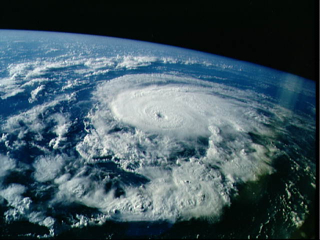
Spacecraft are excellent vantage points from which to observe tropical cyclones. A beautiful example is Hurricane Bonnie, photographed over the western Atlantic from a space shuttle (Figure 1.7). Note the central dense cloud mass, which represents the core of the storm where air is rising and water vapor is condensing into cloud droplets, which combine to form precipitation. This central cloud mass may be from 100 km to as much as 600 km in diameter. Most (but not all) tropical cyclones that reach hurricane intensity have central clear regions, called ``eyes"; these range in diameter from 20 km to as much as 200 km. An eye is clearly visible in Hurricane Bonnie (Figure 1.7). Note also the spiral bands of cumulus and cumulonimbus cloud extending out to as much as 1000 km from the storm center. The tallest clouds in these bands also extend most or all of the way through the depth of the troposphere. The passage of spiral bands at the surface is usually accompanied by strong and gusty winds and sharp showers or thunderstorms. The opaque cloud that comprises the central dense overcast consists of one or more rings of cumulonimbus cloud capped by dense layers of altostratus and cirrostratus (the latter is composed of ice crystals). Click here to go to a gallery of tropical cyclone pictures from space.
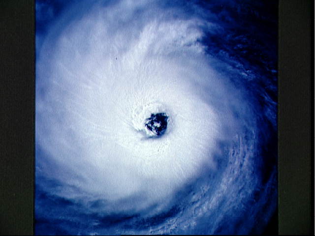
Figure 1.8 shows a close-up of the eye of Hurricane Fefa, in the eastern North Pacific, also photographed from a space shuttle. The funnel-shaped eye is surrounded by a ring of intense and turbulent cumulonimbus, comprising the eyewall. As we shall see later, most of the interesting physics occurs in and under the eyewall and in the eye. Also note that scattered stratocumulus clouds often cover the base of the eye, only a few hundred meters above the highly agitated ocean surface.
Satellites have proven to be an enormous benefit for the detection and monitoring of tropical cyclones, especially as they form and live most of their lives over tropical oceans, where other observations are scarce. Before satellite observation became routine in the 1960's, many storms escaped detection altogether. For example, it was thought that hurricanes were rare in the eastern North Pacific region, because very few of them ever strike land and there is little shipping in the area. We now know that the tropical eastern North Pacific has the highest incidence of storms per unit area per unit time anywhere on earth, during July and August. There are also many techniques for estimating quantitatively certain aspects of storm structure and intensity. Passive infrared radiometers sense upwelling radiation, which is affected by the vertical distribution of temperature and longwave emitters such as water vapor, carbon dioxide and clouds. By measuring the upwelling radiation in several spectral windows, one can make inferences about certain weighted vertical integrals of atmospheric temperature. As we shall soon see, the eyes of tropical cyclones are very warm compared to their surroundings, and this relative warmth can be estimated using passive infrared measurements from space. This is a central component of the Dvorak Technique for estimating tropical cyclone intensity from space. (A thorough description of this technique may be found in WMO (1993) [9], which is a comprehensive tropical cyclone forecaster's handbook.) Occasionally, active sea surface scatterometers are flown on polar orbiting satellites. These instruments operate by transmitting pulses of microwave radiation down to the surface, where some of the radiation is backscattered to a receiver on the satellite. The wavelength of the radiation is chosen to be near the scale of capillary waves on the sea surface, so that the intensity of the backscattered radiation is sensitive to the amplitude and orientation such waves. As the satellite moves, it transmits radiation in at least two different directions, so that each point on the surface is viewed from at least two different angles. By this means, the amplitude and orientation of the capillary waves can be estimated. Since capillary wave amplitude is directly proportional to surface wind stress, a good estimate of surface wind direction and speed can be made. Figure 1.9 shows an example of surface wind distributions around a tropical cyclone, obtained from a satellite-borne scatterometer. Another technique for estimating wind speed is to measure another set of microwave spectral bands in radiation upwelling form the surface itself, as well as the atmosphere. The magnitude of this radiation is sensitive to the surface emissivity as well as water vapor and condensed water in the atmosphere. By measuring in several spectral windows, the effects of water vapor and condensed water can be filtered out to yield an estimate of the surface emissivity, which in the case of a water surface, is a function of the character of the surface, which is in turn related to wind speed. Also, integral measures of atmospheric water vapor content and precipitation rates can be estimated. Another very useful instrument is meteorological radar, and one has just been mounted on a satellite as part of the Tropical Rainfall Measurement Mission (TRMM). This transmits pulses of microwave radiation that is then backscattered by precipitation in the atmosphere, yielding estimates of the distribution of precipitation in three dimensions. Since the fall speed of precipitation is a function of the size of the drops, and the reflectivity is sensitive to the size, an estimate of the precipitation rate can also be made. The very first image transmitted back to earth from the TRMM satellite captured a South Pacific tropical cyclone, as shown in Figure 1.10. The cross-section shows the radar reflectivity, a measure of the precipitation content.
In spite of the enormous usefulness of remote sensing measurements from space, much of what we know about the detailed thermal and kinematic structure of tropical cyclones is derived from direct measurements from aircraft and from airborne Doppler radar data. Aircraft reconnaissance of tropical cyclones began in the late 1940s and has been performed routinely in virtually all Atlantic tropical cyclones of tropical storm strength or greater, since the 1950s. Reconnaissance is carried out by the U.S. Air Force, using C-130 turboprop aircraft, and by the National Oceanographic and Atmospheric Administration (NOAA), now using WP-3D Orion turboprop aircraft as well as a Gulfstream IV jet aircraft. The C-130's and WP-3D's can fly as high as about 8 km, while the Gulfstream IV, which began active duty in 1997, can fly up to about 14 km. (In the 1960's, high-flying military aircraft operated by the U.S. also made measurements up to about 14 km.) Aircraft reconnaissance was also performed in the northwest Pacific region by the U.S. Navy up through 1987. Aircraft reconnaissance is relatively safe, and although a few planes were lost early in the program, there have been no serious accidents in many years.
Aircraft can make direct measurements of temperature, pressure, water vapor and condensed phase water, and by measuring airspeed and ground-relative wind from inertial instruments or the Global Positioning System (GPS), the horizontal components of the wind speed may be deduced. (In the late 1950s and early 1960s, a Doppler radar pointed down at an angle to the sea surface was used to estimate the aircraft ground-relative velocity.) Aircraft also deploy instrument packages called dropwindsondes, which float down to the sea surface on parachutes, measuring wind, temperature and moisture on the way. This gives vertical profiles of these quantities beneath the aircraft flight level. On some occasions, Aircraft-deployed Expendable Bathythermographs (AXBT's) are used. Like dropwindsondes, these float down to the sea surface on parachutes, but once there, a wire spool is deployed from the sonde, which floats on the sea surface. The spool unwinds to a depth of up to 100 m or so and has thermistors deployed along its length. These transmit information on temperature and, sometimes, salinity back to the sonde which in turn transmits the information back to the aircraft by radio. In this way, the thermal structure of the upper ocean can be measured.
The kinematic and thermal structure of a particular Atlantic storm, Hurricane
Inez, is shown in Figure 1.11, Figure 1.12, Figure 1.13 and Figure 1.14, from
Hawkins and Imbembo (1976) [6]. Hurricane Inez was a small but intense
storm, located off the east coast of Florida at the time these measurements were
made. The horizontal distribution of low-level wind speed is shown in
Figure 1.11. (Note that the horizontal coordinates of this diagram are in
nautical miles. One nautical mile is equal to 1852 meters. Also note that the
wind speeds are in nautical miles per hour, or ``knots". One knot = 0.5144
m/s.) The near circular symmetry of the wind field is apparent, though some
asymmetries are evident in the outer region. The wind speed increases gradually
(roughly as  up to a crescent-shaped maximum near the eyewall, then
decreases rapidly, but nearly linearly, to near zero at the storm center. A
vertical cross-section through the storm, again showing the wind speed, can be
seen in Figure 1.12. (Here the vertical coordinate is pressure, not altitude.
The pressure is measured in units of millibars, where one mb = 100 Pascals.
Average surface pressure is 1013 mb. An approximate altitude scale, in feet,
can be seen at the right. The upward bulge of the surface near the storm center
is a consequence of the use of pressure coordinates coupled with the fact that
the surface pressure is much lower in the center of the storm than in its
surroundings.) The dotted lines show the aircraft traverses, and dropwindsondes
were also used to fill in the vertical distributions. Note that the maximum
wind speeds occur very near the surface; this is quite unlike most other
atmospheric wind systems which typically reach maximum amplitude many kilometers
above the surface. The winds fall off very gradually with height at first, but
then more rapidly near the top of the storm. In fact, the sense of rotation
reverses near the top at larger radii form the center. It should be noted,
however, that the wind field near the top of tropical cyclones is rarely very
circularly symmetric.
up to a crescent-shaped maximum near the eyewall, then
decreases rapidly, but nearly linearly, to near zero at the storm center. A
vertical cross-section through the storm, again showing the wind speed, can be
seen in Figure 1.12. (Here the vertical coordinate is pressure, not altitude.
The pressure is measured in units of millibars, where one mb = 100 Pascals.
Average surface pressure is 1013 mb. An approximate altitude scale, in feet,
can be seen at the right. The upward bulge of the surface near the storm center
is a consequence of the use of pressure coordinates coupled with the fact that
the surface pressure is much lower in the center of the storm than in its
surroundings.) The dotted lines show the aircraft traverses, and dropwindsondes
were also used to fill in the vertical distributions. Note that the maximum
wind speeds occur very near the surface; this is quite unlike most other
atmospheric wind systems which typically reach maximum amplitude many kilometers
above the surface. The winds fall off very gradually with height at first, but
then more rapidly near the top of the storm. In fact, the sense of rotation
reverses near the top at larger radii form the center. It should be noted,
however, that the wind field near the top of tropical cyclones is rarely very
circularly symmetric.
The radial component of the wind field is very weak in comparison to the
azimuthal component, except very near the surface and near the top of the storm.
In the atmospheric boundary layer, a layer of air directly affected by surface
friction and by heat fluxes from the surface, the radial wind can be as much as
about 30% of the magnitude of the azimuthal component. This layer is typically
about 1 km thick, but may be much thinner near the eyewall. Vertical velocities
tend to show much finer scale structure than the wind and pressure fields and
are much more difficult to measure. Outside the eyewall, they are dominated by
updrafts and downdrafts associated with convective clouds in the spiral
rainbands, although on average there is a very gentle descent of a few  . The eyewall itself is composed of strong updrafts and some downdrafts,
reaching magnitudes as large as
. The eyewall itself is composed of strong updrafts and some downdrafts,
reaching magnitudes as large as  . On average, the eyewall is a
region of ascent of a few
. On average, the eyewall is a
region of ascent of a few  . Just inside the eyewall, there may be a
sharp downdraft of a few , and inside the eye itself, one typically
finds very gentle descent ( a few ). The strong updrafts in the
eyewall and the strong downdraft just inside the eyewall often give a sharp jolt
to aircraft penetrating the storm. Because the radial and vertical velocity
components are difficult to measure, we defer further discussion of them to a
description of numerical modeling results.
. Just inside the eyewall, there may be a
sharp downdraft of a few , and inside the eye itself, one typically
finds very gentle descent ( a few ). The strong updrafts in the
eyewall and the strong downdraft just inside the eyewall often give a sharp jolt
to aircraft penetrating the storm. Because the radial and vertical velocity
components are difficult to measure, we defer further discussion of them to a
description of numerical modeling results.
Figure 1.13 shows the difference between the measured temperature in the
Hurricane Inez and the temperature at the same pressure in the distant
environment. Clearly, tropical cyclones are ``warm core" phenomena. The
eyewall is typically 2-10 K warmer than the environment, while the center of the
eye itself may be 20 K warmer than the environment. Most of the relative warmth
is concentrated near the top of the storm, while air near the surface is of
nearly uniform temperature. (In fact, some cooling often occurs in the region
of high wind speeds, owing to the evaporation of sea spray and rain.) The
distributions of azimuthal wind and of temperature are directly related in
tropical cyclones, owing to the fact that both the vertical and horizontal
components of the pressure gradient acceleration are nearly balanced by,
respectively, gravity and centrifugal accelerations. When a spatial gradient of
pressure occurs in a fluid, the fluid is accelerated from high to low pressure,
with the rate of acceleration given by  , where
  is the
specific volume of the fluid, which is also the inverse of the fluid
density. Alternatively, in a coordinate system in which pressure
is the
specific volume of the fluid, which is also the inverse of the fluid
density. Alternatively, in a coordinate system in which pressure  is itself
the vertical coordinate, the pressure gradient acceleration can be expressed as
is itself
the vertical coordinate, the pressure gradient acceleration can be expressed as
 , where
  is the geopotential, which is just the
integral of the gravitational acceleration over altitude. The balance condition
for a circular vortex can then be expressed, in pressure coordinates, by the two
equations
is the geopotential, which is just the
integral of the gravitational acceleration over altitude. The balance condition
for a circular vortex can then be expressed, in pressure coordinates, by the two
equations
and
where  is the radial coordinate,
  is the azimuthal velocity, and
 is the Coriolis parameter, defined

where  is the angular velocity of the earth's rotation and
 is the latitude.
The first equation is the hydrostatic equation, reflecting a balance between gravity and an upward-directed pressure gradient acceleration, while the second is called the gradient wind relation, reflecting a balance between the radial pressure gradient acceleration and the sum of the Coriolis and local centrifugal accelerations acting on the wind. These two relations are very well satisfied in tropical cyclones' actual particle accelerations are very small compared to the individual terms in (1) and (2). We also have the ideal gas law:
where  is a gas constant for dry air and
  is temperature.
(Note that (3) is not exact, owing to the effect of variable water
content on density.) Now if we eliminate by cross-differentiating
()eq:1 and (2), and we use (3) for
is temperature.
(Note that (3) is not exact, owing to the effect of variable water
content on density.) Now if we eliminate by cross-differentiating
()eq:1 and (2), and we use (3) for  , we get
Thus the inward-directed temperature gradient is directly associated with the
upward decrease in azimuthal winds. The maximum radial temperature gradient is
near the eyewall, where the upward decrease of is greatest and where  is also largest.
A thermodynamic quantity of great significance for understanding the energy
cycle of tropical cyclones is the specific entropy,  . This can be defined as
a weighted average of the specific entropies of dry air, water vapor and liquid
water in a sample containing all three and for which it is assumed that the
liquid and vapor phases of water are in equilibrium. (Of course, the ice phase
is also prominent in tropical cyclones, but the latent heat of fusion is
somewhat smaller than that of vaporization, so in the first approximation we
neglect it.) Thus we may write
. This can be defined as
a weighted average of the specific entropies of dry air, water vapor and liquid
water in a sample containing all three and for which it is assumed that the
liquid and vapor phases of water are in equilibrium. (Of course, the ice phase
is also prominent in tropical cyclones, but the latent heat of fusion is
somewhat smaller than that of vaporization, so in the first approximation we
neglect it.) Thus we may write
where  is the total mass of the sample,
  ,
,  , and
, and  are, respectively, the masses of dry air, water vapor and liquid water in
the sample, and
are, respectively, the masses of dry air, water vapor and liquid water in
the sample, and  ,
,  and
and  are, respectively, the specific
entropies of dry air, water vapor and liquid water. Dividing (5)
through by then gives
are, respectively, the specific
entropies of dry air, water vapor and liquid water. Dividing (5)
through by then gives
where  is the specific humidity, which is the mass of water
vapor per unit mass of air,
is the specific humidity, which is the mass of water
vapor per unit mass of air,  is the specific liquid water content,
and
is the specific liquid water content,
and  is the total specific water content and is equal to
  .
In thermodynamic equilibrium, the Clausius-Clapeyron equation relates the
specific entropies of the vapor and liquid phases:
.
In thermodynamic equilibrium, the Clausius-Clapeyron equation relates the
specific entropies of the vapor and liquid phases:
where  is the latent heat of vaporization of water, and
  is the specific entropy of water vapor in thermodynamic equilibrium with liquid
water. Making use of (7), we may re-write (6) as
is the specific entropy of water vapor in thermodynamic equilibrium with liquid
water. Making use of (7), we may re-write (6) as
We can now use the definitions of the specific entropies of gases and liquids:


and

where and  are the gas constants for dry air and water
vapor, respectively (these are just the universal gas constant divided by the
mean molecular weight of the constituents of dry air and of water in each case),
are the gas constants for dry air and water
vapor, respectively (these are just the universal gas constant divided by the
mean molecular weight of the constituents of dry air and of water in each case),
 is the heat capacity at constant pressure of dry air,
  is the
heat capacity at constant pressure of water vapor,
is the
heat capacity at constant pressure of water vapor,  is the heat
capacity of liquid water,
is the heat
capacity of liquid water,  is the sum of the partial pressures of all the
gases except water vapor, and
is the sum of the partial pressures of all the
gases except water vapor, and  is the partial pressure of water vapor,
generally referred to as the vapor pressure. Using all of these in
(8) gives
is the partial pressure of water vapor,
generally referred to as the vapor pressure. Using all of these in
(8) gives
where  is the relative humidity =
  , where
 is the saturation vapor pressure.
The quantity is conserved following reversible, adiabatic displacements of a
sample of moist air which may also contain cloud water. In a tropical cyclone,
the main source of is turbulent enthalpy flux from the ocean to the
atmosphere, while the main sink is radiative cooling to space. There are also
irreversible entropy sources owing to dissipation of kinetic energy, to
evaporation of rain and snow in subsaturated air, and to surface evaporation
into subsaturated air.
In meteorology, it is conventional to define another quantity closely related to
the entropy, , called the equivalent potential temperature,  .
It is related to by
.
It is related to by
where the last term is an integration constant and  is a
reference pressure, usually taken to be 1000 mb. Note from (10) that
is a
reference pressure, usually taken to be 1000 mb. Note from (10) that
 has the units of temperature.
Figure 1.14 shows the distribution of  is Hurricane Inez. There are
several very important aspects of the distribution of
is Hurricane Inez. There are
several very important aspects of the distribution of  to note in
Figure 1.14. First, notice that near the edges of the diagram, in the outer
regions of the storm,
to note in
Figure 1.14. First, notice that near the edges of the diagram, in the outer
regions of the storm,  decreases upward from the sea surface to
roughly 600 mb., and then increases with altitude. This is a characteristic of
all convecting atmospheres, of which the tropical atmosphere is a prominent
example. Travelling inward along the surface, note that gradients of
decreases upward from the sea surface to
roughly 600 mb., and then increases with altitude. This is a characteristic of
all convecting atmospheres, of which the tropical atmosphere is a prominent
example. Travelling inward along the surface, note that gradients of  are weak and irregular until one reaches the very high wind speed core, at which
point
are weak and irregular until one reaches the very high wind speed core, at which
point  increases inward very sharply, reaching a maximum value in the
eye. Also notice that in the eyewall region, surfaces of constant
increases inward very sharply, reaching a maximum value in the
eye. Also notice that in the eyewall region, surfaces of constant  are nearly vertical, but flare out to large radii in the upper troposphere.
Supposing for the time being that Hurricane Inez existed in a nearly steady
state at the time these measurements were made, let's imagine the history of
 in a sample of air starting near the surface in the outer regions of
the storm, in Figure 1.14. As it spirals inward toward the eyewall, there is at
first very little change in its
in a sample of air starting near the surface in the outer regions of
the storm, in Figure 1.14. As it spirals inward toward the eyewall, there is at
first very little change in its  , although irregular fluctuations do
occur. Then, as it enters the region of very strong winds near the eyewall, it
undergoes a rapid increase in its entropy (
, although irregular fluctuations do
occur. Then, as it enters the region of very strong winds near the eyewall, it
undergoes a rapid increase in its entropy ( ). This is owing to very
large heat transfer from the ocean, in association with the terrific wind speeds
in the eyewall, and to some extent also to large dissipation of the kinetic
energy of the winds associated with surface friction and high levels of
turbulence. At this point, the airflow abruptly turns upward into the ring of
cumulonimbus clouds comprising the eyewall. As the air flows up the eyewall, it
very nearly conserves its entropy and so flows along surfaces of constant
). This is owing to very
large heat transfer from the ocean, in association with the terrific wind speeds
in the eyewall, and to some extent also to large dissipation of the kinetic
energy of the winds associated with surface friction and high levels of
turbulence. At this point, the airflow abruptly turns upward into the ring of
cumulonimbus clouds comprising the eyewall. As the air flows up the eyewall, it
very nearly conserves its entropy and so flows along surfaces of constant
 . (As water vapor condenses into liquid water in the eyewall, there
are large conversions between latent and sensible heat, but this does not affect
the total specific entropy content.) In the upper troposphere, the airflow
begins to turn outward, still conserving its entropy and thus still following
surfaces of constant
. (As water vapor condenses into liquid water in the eyewall, there
are large conversions between latent and sensible heat, but this does not affect
the total specific entropy content.) In the upper troposphere, the airflow
begins to turn outward, still conserving its entropy and thus still following
surfaces of constant  . Effectively, the entropy gained from the sea
surface is exported to the far environment of the storm, where it is eventually
lost by radiative cooling.
. Effectively, the entropy gained from the sea
surface is exported to the far environment of the storm, where it is eventually
lost by radiative cooling.
It will be helpful to remember this entropy budget later when we discuss the energetics of mature tropical cyclones. In the next lecture, we shall discuss the physics of the tropical atmosphere, which is the breeding ground of tropical cyclones.


